Hyuksoo

1. Introduction

The Nepal earthquake of 2015 (also known as the Gorkha Earthquake) was a catastrophic earthquake that struck near the city of Kathmandu and resulted in around 9,000 casualties and more than 600,000 buildings being structurally damaged. Following the earthquake, Nepal carried out a survey to assess building damage in the earthquake-affected districts. The survey data was open to the public through the 2015 Nepal Earthquake Open Data Portal and is one of the largest post-disaster datasets collected with information on earthquake impact, household conditions, and socio-economic demographics.

Our team competed in the “Richter’s Predictor: Modeling Earthquake Damage” challenge hosted by DrivenData , which prompts competitors to use the data from this survey to develop the best statistical model for predicting the level of damage sustained by different buildings. There are three levels of structural damage to predict: (1) low damage, (2) medium damage, and (3) near-complete destruction. In order to produce the best results, a series of classification models were built and tuned to optimize the accuracy of damage prediction.

Jupyter Notebook for EDA

Jupyter Notebook for Model

Jupyter Notebook for Feature Engineering

2. Data Exploration

The dataset was made publicly available by Nepal’s government following a survey conducted between January 2016 and May 2016. It consists of 347,469 rows and 39 numeric and categorical columns that provide information about a building such as structure and dimensions of building, structural materials of building, building usage, and more.

Number of observation: 347,469 (train: 260,601 | test: 86,868)
Dependent variables: 39
Number of classes: 3 -level of damage (1: low, 2: medium, 3: high)
Missing values: none

The data exploration process started with categorizing the variables into four factors that were hypothesized to have a relationship with damage level. The categories were geography, building structure, building materials, and building usage.

Geography: train_values - column 1:3 - 'geo_level_1_id' ~ 'geo_level_3_id'
Building structure: train_values - column 4:14 - 'count_floors_pre_eq' ~ 'plan_configuration'
Building materials: train_values - column 15:25 - 'has_superstructure_adobe_mud' ~ 'has_superstructure_other'
Building usage: train_values - column 26:38 - 'legal_ownership_status' ~ 'has_secondary_use_other'

Before starting the modeling process with the data, an initial grasp of the variables and their distributions were desired. In order to do this, a series of exploratory plots were built.

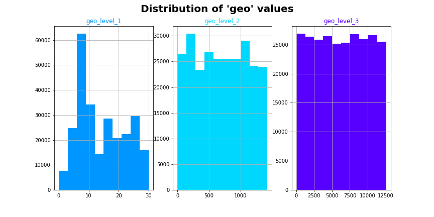
2-1. Geography - Building Location

There were three main geographical variables that represented building location: “geo_level_1_id”, “geo_level_2_id”, and “geo_level_3_id”, which could loosely be interpreted as representing the building’s town (level 1), district (level 2), and street (level 3). Since the values are not coordinate system numbers such as latitude and longitude, they do not provide information on the actual positions of buildings on a map. As such, their encodings provide less interpretability for humans and likely less understandability for a model.

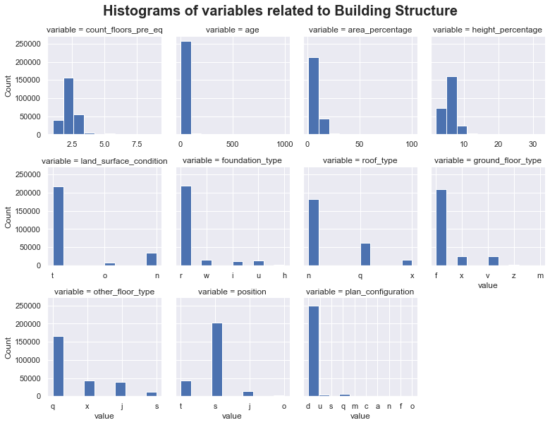
Figure 1. Histograms of variables related to the geographical location of the buildings.

2-2. Building Information

The distributions of numerical and categorical variables show the relatively large imbalance in data across the variables. For example, the 'age' variable, which is a numeric variable of the age of the building in years, includes '999' for age unknown.

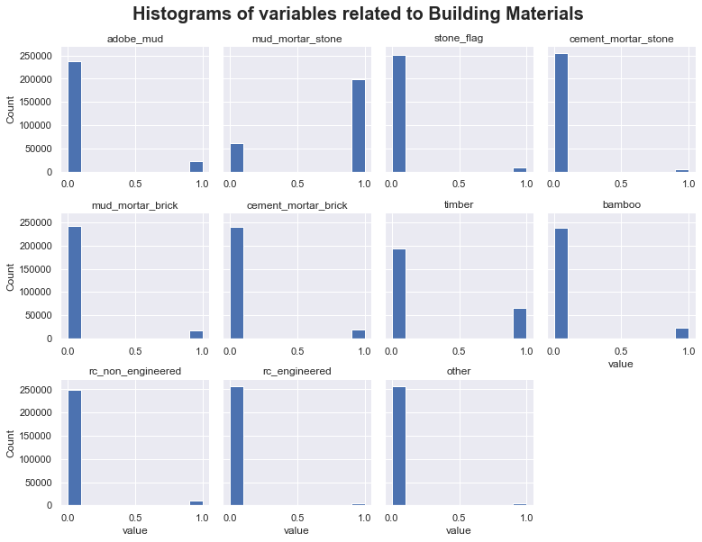
Figure 2. Numerical and categorical variables related to the building structure. This plot shows that some of the variables are skewed towards lower values with some outliers.

The variables related to the building materials are categorical variables and dummy variables are constructed before splitting the dataset.

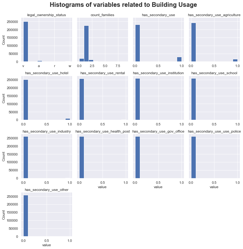
Figure 3. Categorical variables related to the building materials. The plot shows that most of the variables are imbalanced.

The distributions of the secondary use variables are shown and compared to the damage grade levels. Using these visualizations, it is clear that secondary usages have very minimal to zero effect on the damage of a building.

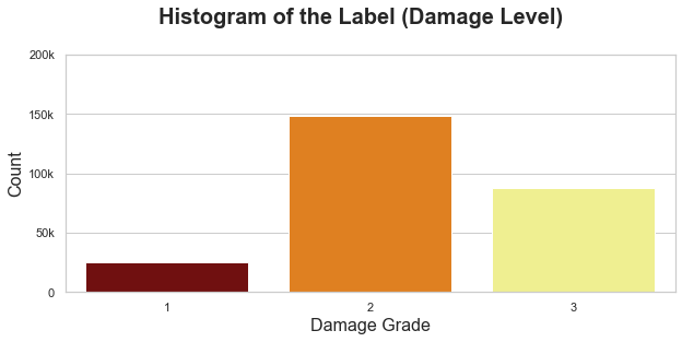
Figure 4. Categorical variables related to the building usage. The plot shows that most of the variables are imbalanced.

2-3. Level of Damage

The plot displays each of the features made available in this competition, including the label. The label, as mentioned above, identifies the level of damage sustained by each building: (1) low, (2) medium, or (3) high.

Figure 5. Distribution of damage level classifications for the training data. There were more training data labeled as "Medium" as compared to "Low" and "High".

3. Model

While there were no missing values across all variables, dummy variables were constructed for the categorical columns and the dataset was split into a 70-30 train-test set. The training and testing sets from this split were established and provided by the DataDriven competition such that the testing set did not contain labels and would be used for final scoring of model submissions. Therefore, all training and testing of models prior to submission had to be done with the given training set in order to assess model accuracy prior to submission. The Random Forest model is used to provide the benchmark for analysis.

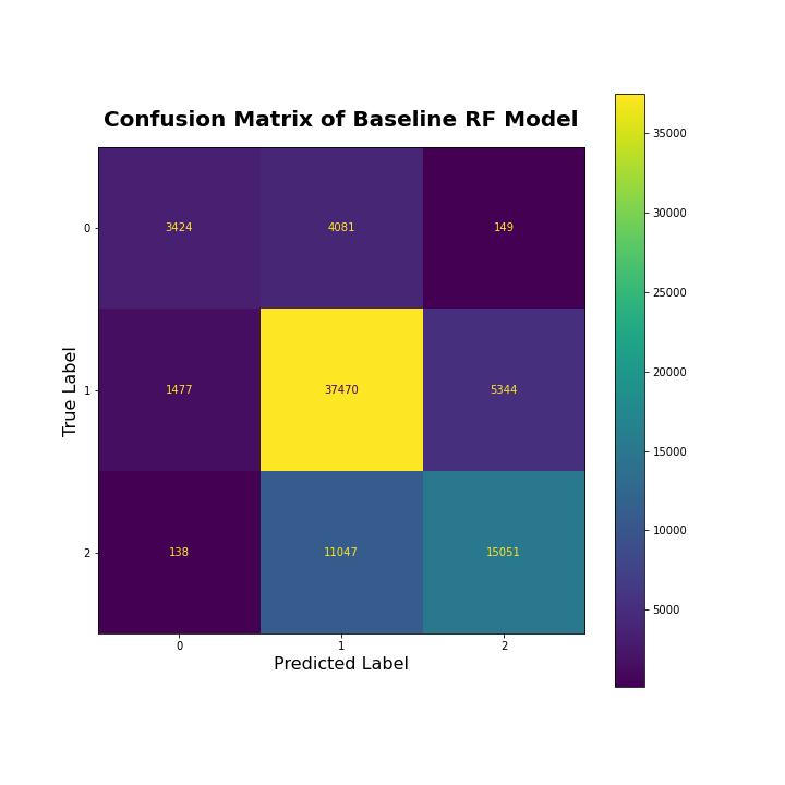
Figure 6. Confusion matrix for Random Forest model (Scikit-learn.ensemble.RandomForestClassifier | Model parameters: n_estimator=150, max_features='sqrt')

It’s seen that almost half of the testing data points were accurately predicted to be of “Medium” damage level. However, of the data that had an actual label of “High”, both models predicted almost half to be “Medium” and the other half to be “High”. This may suggest that these levels of damage have similar criteria seen in the variables. Or, this could be a result of the non-uniform distribution of labels across the training and testing data, and therefore the models did not learn how to distinguish between the majority of data points that were “Medium” damage, and the fewer data points that were “High” damage.

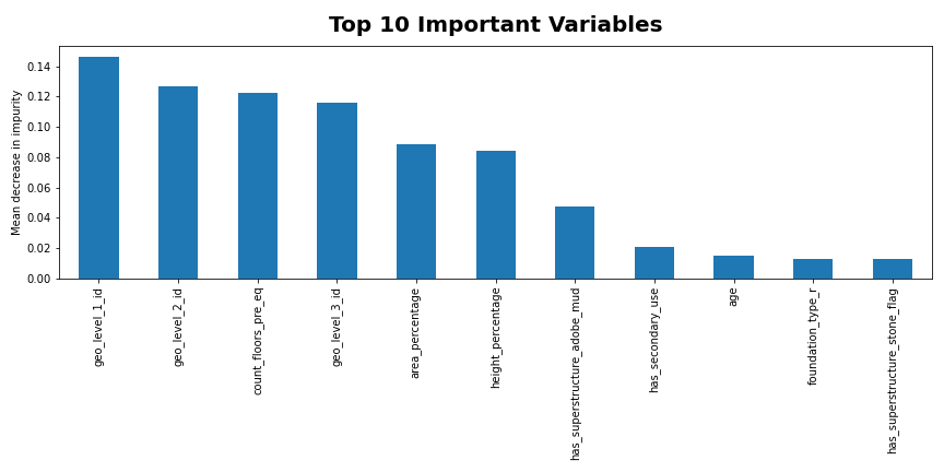
Figure 7. Feature Importance attribute from the Random Forest classifier.

The plot provides insight into the importance of the variables to feature engineer.

4. Feature Engineering

In order to attempt to improve the two best models’ accuracies and to decrease algorithmic complexity, feature engineering was explored in three main ways: feature selection, feature transformation, and feature extraction techniques.

The feature selection process started with categorizing the variables into four factors that were hypothesized to have a relationship with damage level. The categories were geography, building structure, building materials, and building usage. Of these, geography was considered for transformation for two main reasons. First, it is obvious that a building’s location would be an important factor of the level of damage it experiences, as buildings closer to an earthquake’s origin are more likely to experience greater damage. Second, it was seen that the three geographic variables were the top three important variables in all three of the top classification models that were produced without feature engineering: Random Forest, AdaBoost, and Bagging. This is shown and discussed in Figure 6 in the Results section below. Considering these variables’ importance in the pre-feature engineering models, it seemed likely that combining the geographic variables into a single variable may aid in the models’ abilities to interpret and utilize the geographic information.

There were three main geographical variables that represented building location: “geo_level_1_id”, “geo_level_2_id”, and “geo_level_3_id”, which could loosely be interpreted as representing the building’s town (level 1), district (level 2), and street (level 3). These variables simply provided an encoding to represent the building’s street, district, and town. Therefore, since the values are not coordinate system numbers such as latitude and longitude, they do not provide information on the actual positions of buildings on a map. As such, their encodings provide less interpretability for humans and likely less understandability for a model.

To begin the investigation into these variables, a probability table of the geographical regions is created to better connect location data to the level of damage. This process can be thought of as encoding or grouping the area with a similar distance from the origin of the earthquake. Table 1 below shows the table of conditional probabilities created based on geographical variable 1. The “counts” column shows the total number of observations of the geographical identifier. Then, the “damage_1”, “damage_2”, and “damage_3” columns count the intersections of each damage level and the geographical identifier. Finally, the conditional probabilities are calculated by dividing the intersection count, and the results are shown in the last three columns of the table.

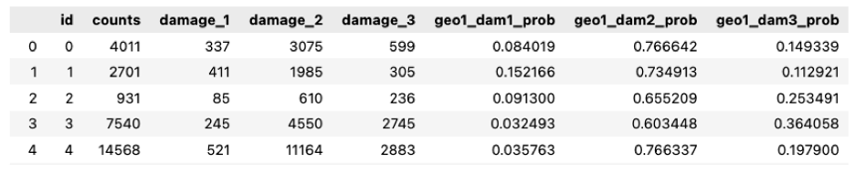
Figure 8. Conditional Probabilities for Geographical Variable 1.

As discussed above, the conditional probabilities shown in Table 1 are calculated using Equation 1, where the frequencies of the intersections are divided by the number of each geographical identifier in the data set.

Based on the above equation and the surrounding discussion, the conditional probabilities can be interpreted as the region-specific risk of damage due to the earthquake. Thus, the geographical variables in the test data set can be readily encoded using Table 1.

Figure 9. Partial Table of the Principal Components Extracted from the Building Material Variables.

With two methods of feature engineering performed, the resulting reduced data set was used to train the top two tuned models: Random Forest and AdaBoost. The results of this are discussed in the following Results section.

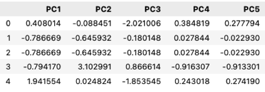
Feature engineering decreased the complexity of the model. Since the variables in the original data set were mostly categorical, a numerical transformation of these categorical variables significantly increased the dimensionality of the data. Therefore, PCA’s ability to decrease the number of variables in the data set allowed for a decrease in complexity. However, further research would be needed to assess the efficiency of applying PCA to binary variables.

5. Result and Conclusion

Performance of the algorithm was measured by a micro-averaged F1 score due to the three possible labels, as opposed to a traditional F1 score that evaluates performance on a binary classifier. The DrivenData competition provided a baseline Random Forest model with an accuracy of 58.15%, 15.93% less accurate than the tuned and feature-engineered Random Forest model produced in this analysis. Also, this analysis’ Random Forest model ranked in the top 10% compared to models produced by more than 5300 other competitors (top score: 75.58%).

Figure 10. Competition Score and Ranking of the Tuned and Feature-Engineered Random Forest Model.

When looking at all of these models and results, many technical conclusions can be drawn regarding the best model for the data, the forecasting accuracy of the model, the important features in the model, and the results from submissions to the competition.

Using this project as a starting point, this could go in many directions. First, using exploratory data analysis, a further in-depth study could reveal more critical relationships between sets of variables and their impact on the damage of buildings. From these discoveries, sets of building codes could be constructed to maximize the safety of buildings in preparation for the next earthquake. Considering earthquakes are not unusual in that region, the next earthquake is bound to cause damage to buildings that were similarly damaged in the previous earthquake.